NFL Redraft
Introduction
At the University of Arkansas, I took a class called Data Analytics Fundamentals in the Fall of 2018, which covered the basics of Microsoft Excel, Microsoft SQL, and Python. The goal of the class was to learn and use these packages to create statistical reports. For the final project, we had to use either SQL or Python to analyze a dataset and present the findings.
The idea for the “NFL Redraft” project came from Twitter, where Namita Nandakumar had released a short presentation on an “NHL Redraft”. The main concept addressed the question of “Who would these teams draft if they knew then what we know now in terms of player performance?”. The main process is going through the draft order for a particular year, with each team selecting the best available player at the position that they actually drafted. Doing this gives a hypothetical draft, which you can then compare to the players actually drafted at those spots. This allows us to analyze which teams significantly outperformed the other teams in a respective draft.
Gathering Data
First, I had to scrape the data (code below) using python (requests_html library), which I got from Pro Football Reference (referred to as PFR going forward). Since I wanted the analysis to be simple, and the hypothetical draft had teams drafting the same position as they did in real life, I decided to use the “Approximate Value” (AV) statistic on PFR. AV attempts to be a one-number summary for the overall value that a player adds to a team. The project asked for all data to be included in a CSV format, so I used pandas to write CSV files.
from requests_html import HTMLSession
import pandas as pd
import numpy as np
session = HTMLSession()

for year in range(2006, 2017):
    url = "https://www.pro-football-reference.com/years/" + str(year) + "/draft.htm"
    page = session.get(url)
    rnd = []
    pick = []
    team = []
    player = []
    position = []
    AV = []
    AV_tm = []
    GP = []
    rd = page.html.find('#drafts th.right')
    pk = page.html.find('#drafts td:nth-child(2)')
    tm = page.html.find('#drafts td:nth-child(3)')
    plr = page.html.find('#drafts td:nth-child(4)')
    pos = page.html.find('#drafts td:nth-child(5)')
    val = page.html.find('#drafts td:nth-child(11)')
    val_tm = page.html.find('#drafts td:nth-child(12)')
    gm = page.html.find('#drafts td:nth-child(13)')
    for i in range(0, len(rd)):
        rnd.append(rd[i].text)
        pick.append(pk[i].text)
        team.append(tm[i].text)
        player.append(plr[i].text)
        position.append(pos[i].text)
        AV.append(val[i].text)
        AV_tm.append(val_tm[i].text)
        GP.append(gm[i].text)
    ## Add exception handling for duplicate names, happens in 2012 draft with "Robert Griffin"
    def list_duplicates(seq):
        seen = set()
        seen_add = seen.add
        return [idx for idx,item in enumerate(seq) if item in seen or seen_add(item)]
    if len(player) != len(set(player)):
        duplicate_name_indices = list_duplicates(player)
        player[duplicate_name_indices[0]] = player[duplicate_name_indices[0]] + " 2"
    draft_df = pd.DataFrame(np.column_stack([rnd, pick, team, player, position, AV, AV_tm, GP]),
                            columns=['Round', 'Pick', 'Team', 'Player', 'Position', 'AV', 'AV_Team', 'GP'])
    filename = "Draft_" + str(year) + ".csv"
    draft_df.to_csv(("./Data/" + filename), index = False)
    print(filename + " written.")
Processing
Now that the data was gathered, the redraft process had to be built. In a fairly simple approach, I iterated through the actual draft order, with the team “selecting” the best player according to AV at the particular position they actually selected in the draft. Since all data had to be in CSV format, I used pandas to export the hypothetical drafts for the analysis step.
import pandas as pd
import numpy as np

for i in range(2006, 2017):
    read_filename = "./Data/Draft_" + str(i) + ".csv"
    draft_full = pd.read_csv(read_filename)
    ## split into structure (picks/team) and available players
    draft_structure = pd.DataFrame(draft_full, columns=['Round', 'Pick', 'Team', 'Position', 'AV'])
    draft_players = pd.DataFrame(draft_full, columns=['Player', 'Position', 'AV', 'GP'])
    drafted_players = ['']
    draft_full['Redraft_Player'] = ""
    draft_full['Redraft_AV'] = np.nan
    for index, row in draft_structure.iterrows():
        ## subsetting based on position and removing all previously drafted players
        pos_subset = draft_players[(draft_players['Position'] == row['Position']) &
                               (draft_players['Player'].isin(drafted_players) == False)]
        ## sorting by AV so best player is drafted (GP is the tiebreaker)
        pos_subset = pos_subset.sort_values(by=['AV', 'GP'], ascending=False)
        drafted_player = pos_subset.iloc[0,0]
        drafted_players.append(drafted_player)
        draft_full.iloc[index, 8] = drafted_player
        draft_full.iloc[index, 9] = pos_subset.iloc[0,2]
    ## export new csv
    write_filename = "Redraft_" + str(i) + ".csv"
    draft_full.to_csv(("./Data/" + write_filename), index = False)
    print(write_filename + " written to Data folder.")
Analysis
Now that I had the information for both the real draft and the hypothetical draft, I brought both into python in order to assess the differences.
results_Eff = pd.DataFrame(columns=['Team', 'Pick_Eff', 'Year'])
results_Diff = pd.DataFrame(columns=['Team', 'Pick_Diff', 'Year'])
results_Eff_rd = pd.DataFrame(columns=['Team', 'Rd' , 'Pick_Eff', 'Count', 'Year'])
results_Diff_rd = pd.DataFrame(columns=['Team', 'Rd', 'Pick_Diff', 'Count' ,'Year'])
for i in range(2006, 2016):
    read_filename = "./Data/Redraft_" + str(i) + ".csv"
    redraft = pd.read_csv(read_filename)
    ## if desired focus on first four rounds since these are the highest impact players
        # redraft = redraft[(redraft['Round']) < 5]
    redraft['Pick_Eff'] = redraft['AV'] / redraft['Redraft_AV']
    redraft['Pick_Diff'] = redraft['AV'] - redraft['Redraft_AV']
    results_Eff_year = redraft.groupby(['Team'])['Pick_Eff'].mean()
    results_Eff_year = pd.DataFrame(results_Eff_year)
    results_Eff_year['Year'] = i
    results_Eff_year.reset_index(inplace=True)
    results_Eff_year.columns = ['Team', 'Pick_Eff', 'Year']
    results_Eff = results_Eff.append(results_Eff_year, ignore_index=True)
    ## Note if running an older version of pandas
        ## A notice will come up asking to put sort = False as an argument for the four append lines
        ## such as results_Eff = results_Eff.append(results_Eff_year, ignore_index=True, sort=False)
        ## I am using a newer version of pandas that has this behavior assumed

    results_Diff_year = redraft.groupby(['Team'])['Pick_Diff'].sum()
    results_Diff_year = pd.DataFrame(results_Diff_year)
    results_Diff_year['Year'] = i
    results_Diff_year.reset_index(inplace=True)
    results_Diff_year.columns = ['Team', 'Pick_Diff', 'Year']
    results_Diff = results_Diff.append(results_Diff_year, ignore_index=True)

    results_Diff_year_rd = redraft.groupby(['Team', 'Round'])['Pick_Diff'].agg(['sum', 'count'])
    results_Diff_year_rd = pd.DataFrame(results_Diff_year_rd)
    results_Diff_year_rd['Year'] = i
    results_Diff_year_rd.reset_index(inplace=True)
    results_Diff_year_rd.columns = ['Team', 'Rd', 'Pick_Diff', 'Count' ,'Year']
    results_Diff_rd = results_Diff_rd.append(results_Diff_year_rd, ignore_index=True)

    results_Eff_year_rd = redraft.groupby(['Team', 'Round'])['Pick_Eff'].agg(['sum', 'count'])
    results_Eff_year_rd = pd.DataFrame(results_Eff_year_rd)
    results_Eff_year_rd['Year'] = i
    results_Eff_year_rd.reset_index(inplace=True)
    results_Eff_year_rd.columns = ['Team', 'Rd' , 'Pick_Eff', 'Count', 'Year']
    results_Eff_rd = results_Eff_rd.append(results_Eff_year_rd, ignore_index=True)
My analysis then answered the following questions:
Which teams performed best in the draft from 2006-2015?
q1 = pd.DataFrame(results_Diff.groupby(['Team'])['Pick_Diff'].sum())
q1.reset_index(inplace = True)
q1.columns = ['Team', 'Total_Differential']
q1 = q1.sort_values(by = ['Total_Differential'], ascending = False)
q1
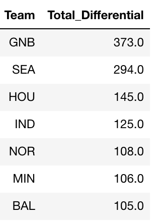
We can see from the results above that the Green Bay Packers appear to have added the most value with their picks. Their total AV differential means that the team added 373 AV through their evaluation and scouting. We can interpret this as the team identifying talent that the rest of the league undervalued. One interesting team in the top 10 teams is the Cincinnati Bengals, who do not have a lot of scouts. This would lead you to believe that their ability to evaluate talent is hampered, but their draft performance indicates they did draft better players at their actual draft positions than we would expect.

Which teams performed worst in the draft from 2006-2015?
q1 = pd.DataFrame(results_Diff.groupby(['Team'])['Pick_Diff'].sum())
q1.reset_index(inplace = True)
q1.columns = ['Team', 'Total_Differential']
q1 = q1.sort_values(by = ['Total_Differential'], ascending = True)
q1
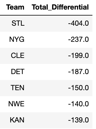
On the other hand, it appears that the St. Louis Rams (now Los Angeles Rams) lost 404 AV through their evaluation of talent, when compared to other teams.

How did teams perform in each year?
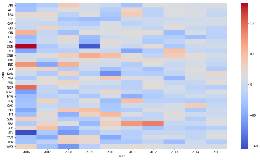
For this question, I chose to use a seaborn heatmap.
import seaborn as sns
import matplotlib.pyplot as plt

plt.figure(figsize=(16, 9))
piv = results_Diff.pivot("Team", "Year", "Pick_Diff")
ax = sns.heatmap(piv, cmap="coolwarm")
First, we see that the earlier years are more likely to be on either extreme. This makes sense, given that the careers of these players have played out more than the players drafted in more recent years. The main takeaway, however, is that there are no teams that consistently underperform or overperform in the draft consistently.
The notable exception is the Green Bay Packers (GNB). They were the best team in terms of draft performance (as addressed earlier), generally outperforming what we would expect, but not in a very extreme manner. This could mean that the teams that do draft well do so over time, which gradually pays off, instead of having one “home run” draft.
Conclusion
Since the careers of players are ongoing, it is important to continually revisit the analysis. If I were to do this analysis again, I would focus on a range of years slightly older than used here. This would provide a more conclusive result, since the heatmap shows that more recent years are not as well defined as good or bad.